How to see duplicates in excel. Duplicate values ​​in Excel - find, highlight or remove duplicates in Excel

Miscellaneous (39)
Excel bugs and glitches (3)

How to get a list of unique (non-repeated) values?

Imagine a large list of various names, full names, personnel numbers, etc. And it is necessary to leave a list of all the same names from this list, but so that they do not repeat - i.e. remove all duplicate entries from this list. As it is otherwise called: create a list of unique elements, a list of non-repeating, no duplicates. There are several ways to do this: using built-in Excel tools, built-in formulas, and finally using code. Visual Basic for Application(VBA) and pivot tables. In this article, we'll take a look at each option.

Using the built-in capabilities of Excel 2007 and later
In Excel 2007 and 2010, this is easy to do - there is a special command, which is called -. It is located on the tab Data subsection Working with data (Data tools)

How to use this command. Highlight a column (or several) with the data in which you want to remove duplicate entries. Go to tab Data -Remove Duplicates.

If you select one column, but next to it there are more columns with data (or at least one column), then Excel will offer you a choice: expand the selection range with this column or leave the selection as it is and delete data only in the selected range. It is important to remember that if you do not expand the range, then the data will change only in one column, and the data in the adjacent column will remain unchanged.

A window will appear with options for removing duplicates.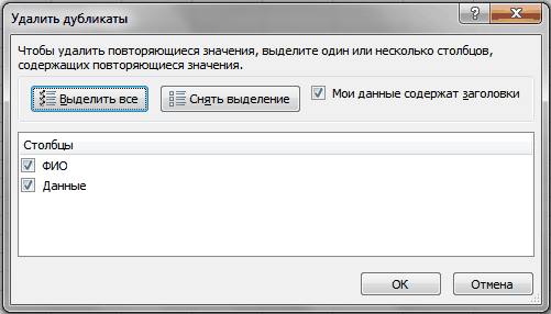

Check the boxes next to the columns in which you want to remove duplicates and click OK. If the selected range also contains data headers, then it is better to set the flag My data contains headers so as not to accidentally delete data in the table (if they suddenly completely match the value in the header).

Method 1: Advanced filter
In the case of Excel 2003, everything is more complicated. There is no such tool as Remove Duplicates. But there is such a wonderful tool as Advanced filter. In 2003 this tool can be found in Data -Filter -Advanced filter. The beauty of this method is that with its help you can not spoil the original data, but create a list in a different range. In 2007-2010 Excel, it is also there, but a little hidden. Located on tab Data, group Sort & Filter - Advanced
How to use it: run the specified tool - a dialog box appears:

• Treatment: Choose Copy the result to another location (Copy to another location).
• Source range (List range) : Selecting a range with data (in our case it is A1:A51).
• Criteria range : in this case, leave it blank.
• Put the result in a range (Copy to) : specify the first cell for data output - any empty (in the picture - E2).
• Put a tick Only unique records (Unique records only).
• Click OK.

Note: if you want to put the result on another sheet, then just specifying another sheet will not work. You will be able to specify a cell on another sheet, but... Alas and ah... Excel will display a message that it cannot copy the data to other sheets. But this can be bypassed, and quite simply. You just need to run Advanced filter from the sheet on which we want to place the result. And as the initial data, we select data from any sheet - this is allowed.

You can also not transfer the result to other cells, but filter the data in place. The data will not suffer from this in any way - it will be a normal data filtering.

To do this, simply select in the Processing section Filter the list, in-place.

Method 2: Formulas
This method is more difficult to understand for inexperienced users, but it creates a list of unique values ​​without changing the original data. Well, it is more dynamic: if you change the data in the source table, the result will also change. Sometimes this is useful. I'll try to explain on my fingers what's what: let's say your list with data is located in column A (A1: A51, where A1 is the heading). We will display the list in column C, starting from cell C2. The formula in C2 would be:
(=INDEX($A$2:$A$51 ;SMALL(IF(COUNTIF($C$1:C1 ; $A$2:$A$51)=0;ROW($A$1:$A$50));1)) )
(=INDEX($A$2:$A$51 ;SMALL(IF(COUNTIF($C$1:C1 ; $A$2:$A$51)=0;ROW($A$1:$A$50));1)) )
A detailed analysis of the work of this formula is given in the article:
Note that this formula is an array formula. This can be indicated by the curly brackets in which this formula is enclosed. And the following formula is entered into the cell with a keyboard shortcut - ctrl+Shift+Enter. After we have entered this formula in C2, we must copy and paste it on several lines so that all unique elements are accurately displayed. Once the formula in the bottom cells returns #NUMBER!- this means all the elements are displayed and there is no point in stretching the formula below. To avoid an error and make the formula more universal (without stretching each time until an error occurs), you can use a simple check:
for Excel 2007 and above:
(=IFERROR(INDEX($A$2:$A$51 ,SMALL(IF(COUNT($C$1:C1 , $A$2:$A$51)=0,ROW($A$1:$A$50)),1 ));""))
(=IFERROR(INDEX($A$2:$A$51 ;SMALL(IF(COUNTIF($C$1:C1 ; $A$2:$A$51)=0;ROW($A$1:$A$50));1 ));""))
for Excel 2003:
(=IF(ISN(SMALL(IF(COUNTIF($C$1:C1 , $A$2:$A$51)=0,ROW($A$1:$A$50)),1)),"";INDEX( $A$2:$A$51 ;SMALL(IF(COUNT($C$1:C1 ; $A$2:$A$51)=0;ROW($A$1:$A$50));1))))
(=IF(ISERR(SMALL(IF(COUNTIF($C$1:C1 ; $A$2:$A$51)=0;ROW($A$1:$A$50));1));"";INDEX( $A$2:$A$51 ;SMALL(IF(COUNTIF($C$1:C1 ; $A$2:$A$51)=0;ROW($A$1:$A$50));1))))
Then instead of an error #NUMBER! (#NUM!) you will have empty cells (not completely empty, of course - with formulas :-)).

A little more about the differences and nuances of the IFERROR and IF(EOSH) formulas can be found in this article: How to show 0 instead of an error in a cell with a formula

Method 3: VBA code
This approach will require the permission of macros and basic knowledge about working with them. If you are not sure about your knowledge, I recommend reading these articles first:

• What is a macro and where can I find it? video tutorial attached to the article
• What is a module? What are the modules? required to understand where to insert the codes below

Both of the following codes should be placed in standard module. Macros must be enabled.

We will leave the initial data in the same order - the list with the data is located in column "A" (A1:A51 where A1 is the title). Only we will display the list not in column C, but in column E, starting from cell E2:

Sub Extract_Unique() Dim vItem, avArr, li As Long ReDim avArr(1 To Rows.Count, 1 To 1) With New Collection On Error Resume Next For Each vItem In Range("A2", Cells(Rows.Count, 1) .End(xlUp)).Value "Cells(Rows.Count, 1).End(xlUp) - defines the last filled cell in column A. Add vItem, CStr(vItem) If Err = 0 Then li = li + 1: avArr(li, 1) = vItem Else: Err.Clear End If Next End With If li Then .Resize(li).Value = avArr End Sub

Using this code, you can extract unique ones not only from one column, but also from any range of columns and rows. If instead of the line
Range("A2", Cells(Rows.Count, 1).End(xlUp)).Value !}
specify Selection.Value , then the result of the code will be a list of unique elements from the range selected on the active sheet. Only then it would be nice to change the value output cell - instead of put the one in which there is no data.
You can also specify a specific range:

Range("C2", Cells(Rows.Count, 3).End(xlUp)).Value

Generic code for selecting unique values
The code below can be applied to any ranges. It is enough to run it, specify a range with values ​​for selecting only non-repeating ones (more than one column is allowed) and a cell for displaying the result. The specified cells will be scanned, only unique values ​​will be selected from them (empty cells are skipped) and the resulting list will be written starting from the specified cell.

Sub Extract_Unique() Dim x, avArr, li As Long Dim avVals Dim rVals As Range, rResultCell As Range On Error Resume Next "request the address of the cells to select unique values Set rVals = Application.InputBox( "Specify a range of cells to sample unique values", "Query Data" , "A2:A51" , Type :=8) If rVals Is Nothing Then "if the Cancel button is pressed Exit Sub End If "if only one cell is specified, there is no point in choosing If rVals.Count = 1 Then MsgBox "More than one cell is required to select unique values", vbInformation, "www.site" Exit Sub End If "cut off empty rows and columns outside the working range Set rVals = Intersect(rVals, rVals.Parent.UsedRange) "if only empty cells outside the working range are specified If rVals Is Nothing Then MsgBox "Insufficient data to select values", vbInformation, "www.site" Exit Sub End If avVals = rVals.Value "request a cell to display the result Set rResultCell = Application.InputBox( "Specify a cell to insert selected unique values", "Query Data" , "E2" , Type :=8) If rResultCell Is Nothing Then "if the Cancel button is pressed Exit Sub End If "define the maximum possible array size for the result ReDim avArr(1 To Rows.Count, 1 To 1) "using the Collection object "select only unique records, "because Collections cannot contain duplicate values With New Collection On Error Resume Next For Each x In avVals If Len(CStr(x)) Then "skip empty cells.Add x, CStr(x) "if the element being added is already in the Collection, an error will occur "if there is no error - such a value has not yet been entered, "add to the resulting array If Err = 0 Then li = li + 1 avArr(li, 1) = x Else "be sure to clear the Errors object Err.Clear End If End If Next End With "write the result to the sheet, starting from the specified cell If li Then rResultCell.Cells(1, 1).Resize(li).Value = avArr End Sub

Sub Extract_Unique() Dim x, avArr, li As Long Dim avVals Dim rVals As Range, rResultCell As Range On Error Resume Next , "Query data", "A2:A51", Type:=8) If rVals Is Nothing Then "if the Cancel button is pressed Exit Sub End If "if only one cell is specified, it makes no sense to select If rVals.Count = 1 Then MsgBox " To select unique values, you need to specify more than one cell", vbInformation, "www.site" Exit Sub End If "cut off empty rows and columns outside the working range Set rVals = Intersect(rVals, rVals.Parent.UsedRange) "if only empty cells are specified out of range If rVals Is Nothing Then MsgBox "Insufficient data to select values", vbInformation, "www..Value "request a cell to display the result Set rResultCell = Application.InputBox("Укажите ячейку для вставки отобранных уникальных значений", "Запрос данных", "E2", Type:=8) If rResultCell Is Nothing Then "если нажата кнопка Отмена Exit Sub End If "определяем максимально возможную размерность массива для результата ReDim avArr(1 To Rows.Count, 1 To 1) "при помощи объекта Коллекции(Collection) "отбираем только уникальные записи, "т.к. Коллекции не могут содержать повторяющиеся значения With New Collection On Error Resume Next For Each x In avVals If Len(CStr(x)) Then "пропускаем пустые ячейки.Add x, CStr(x) "если добавляемый элемент уже есть в Коллекции - возникнет ошибка "если же ошибки нет - такое значение еще не внесено, "добавляем в результирующий массив If Err = 0 Then li = li + 1 avArr(li, 1) = x Else "обязательно очищаем объект Ошибки Err.Clear End If End If Next End With "записываем результат на лист, начиная с указанной ячейки If li Then rResultCell.Cells(1, 1).Resize(li).Value = avArr End Sub!}

Method 4: Pivot Tables
Somewhat non-standard way to extract unique values.

• Select one or more columns in the table, go to the tab Insert-group Table -PivotTable
• In the dialog box Creating a PivotTable (Create PivotTable) check the correctness of the selection of the data range (or install a new data source)
• specify the location of the PivotTable:
  • To a new sheet (New Worksheet)
  • To an Existing Worksheet
• confirm the creation by pressing the button OK

Because Pivot tables, when processing data that are placed in the rows or columns area, select only unique values ​​​​from them for further analysis, then absolutely nothing is required of us, except to create a pivot table and place the data of the desired column in the rows or columns area.
Using the example of the file attached to the article, I:

What is the inconvenience of working with pivot tables in this case: when changing in the source data, the pivot table will have to be updated manually: Select any cell of the pivot table -Right mouse button - Refresh or tab Data -Refresh all -Refresh. And if the initial data is replenished dynamically and even worse - it will be necessary to re-specify the range of the initial data. And one more minus - the data inside the pivot table cannot be changed. Therefore, if it will be necessary to work with the resulting list in the future, then after creating the desired list using the summary, it must be copied and pasted onto the desired sheet.

In order to better understand all the actions and learn how to handle pivot tables, I strongly recommend that you read the article Overview of Pivot Tables - a video tutorial is attached to it, in which I clearly demonstrate the simplicity and convenience of working with the main features of pivot tables.

In the attached example, in addition to the described techniques, a slightly more complex variation of extracting unique elements with a formula and code is recorded, namely: extracting unique elements by criteria. What is it about: if in one column of the surname, and in the second (B) there is some data (in the file these are months) and it is required to extract the unique values ​​of column B only for the selected surname. Examples of such unique extractions are located on the sheet Extract by criteria.

Download example:

(108.0 KiB, 14,501 downloads)

Did the article help? Share the link with your friends! Video lessons

Microsoft Excel is quite rich in the functions of analyzing data ranges, earlier we considered how you can, how you can use it for two data ranges, as well as the visualization of statistical information with the addition of a function.

Today we will talk about how to find duplicate values ​​in Excel tables. The method presented in the article will be based on the use of conditional formatting. In fact, there will be two ways - one is general, which will help you better understand the basic principles of conditional formatting, and the second is simple.

See also the video version of the article.

The first part of the method

Consider an example of finding duplicate values.

To find duplicate values, do the following step by step algorithm actions:

1. Select source range (A1:E8)
2. Run command: Home tab / Styles group / Conditional Formatting / Create Rule

1. In the dialog box, select: “Use a formula to determine formatted cells”, while the dialog box will change its appearance a little, then enter the following formula: =COUNTIF($A$1:$E$8,A1)>1

   after entering the formula, you must select the format that will be applied to the cells that satisfy the condition (in the example, the fill is orange).

1. After pressing the "OK" button, you can immediately observe the result of the operation.

The entered formula compares the value of each individual cell with cells from the range and, if the cell is not unique, then formatting is applied to it, in our case, the cell is filled with orange.

Second part of the method.

Sometimes it becomes necessary to search not for repeating cells, but for entire rows.

1. The main idea of ​​finding non-unique, or, conversely, unique strings, is to make one of all the strings in the range by concatenation (connection), and then look for non-unique values ​​in the new range. By the way, you can also join strings in more than one way, for example, the concatenation sign “&” is perfect, as well as the function .

1. The next step is to search for non-unique rows among the new column, the selection of the cells of which will show the duplicate rows in the original table. The search, as in the first part of the method, could be performed with the construction of a formula, but it can be made simpler.

In the window for constructing MS Excel rules, the developers have already provided for the most common scenarios for using this tool, so you can not enter the formula, but select the item " Format only unique or duplicate values»

1. After clicking "OK", the result will not be long in coming.

Finally, it should be mentioned that conditional formatting works dynamically, i.e. If certain values in non-unique strings will be changed in such a way that the strings become unique, then the formatting will automatically change. The reverse is also true.

Finding duplicates in Excel is one of the most common tasks for any office worker. To solve it, there are several different ways. But how to quickly find duplicates in Excel and highlight them with color? To answer this frequently asked question, consider a specific example.

How to find duplicate values ​​in Excel?

Suppose we are engaged in the registration of orders received by the company via fax and e-mail. There may be such a situation that the same order was received by two channels of incoming information. If you register the same order twice, certain problems may arise for the company. Below is a solution using conditional formatting.

To avoid duplicate orders, you can use conditional formatting to help you quickly find duplicate values ​​in an Excel column.

Example of a daily log of orders for goods:

To check if the order log contains possible duplicates, we will analyze by customer names - column B:

As you can see in the figure with conditional formatting, we were able to easily and quickly implement duplicate search in Excel and detect duplicate cell data for the order history table.



COUNTIF example and highlighting duplicate values

The principle of the formula for finding duplicates by conditional formatting is simple. The formula contains the function =COUNTIF(). This function can also be used when searching for the same values ​​in a range of cells. The first argument in the function is the data range to be viewed. In the second argument, we specify what we are looking for. The first argument we have has absolute references, since it must be immutable. And the second argument, on the contrary, should change to the address of each cell of the viewed range, therefore it has a relative link.

The fastest and simple ways: find duplicates in cells.

The function is followed by an operator for comparing the number of found values ​​in the range with the number 1. That is, if there is more than one value, then the formula returns TRUE and conditional formatting is applied to the current cell.

If you are working with large numbers information in Excel and regularly add it, for example, data about school students or company employees, then duplicate values ​​may appear in such tables, in other words, duplicates.

In this article, we will look at how to find, select, delete and count the number of duplicate values ​​in Excel.

How to find and highlight

You can find and highlight duplicates in a document using conditional formatting in Excel. Select the entire range of data in the desired table. On the Home tab, click the button "Conditional Formatting", choose from the menu "Cell Selection Rules" – "Duplicate Values".

In the next window, select from the dropdown list "recurring", and the color for the cell and the text to fill in the found duplicates. Then click "OK" and the program will search for duplicates.

In the Excel example, all the same information is highlighted in pink. As you can see, the data is not compared line by line, but highlighted identical cells in columns. Therefore, the cell "Sasha V." . There may be several such students, but with different surnames.

How to count

If you need to find and count the number of duplicate values ​​in Excel, we will create a summary for this Excel spreadsheet. Add to the original column "Code" and fill it with "1": put 1, 1 in the first two cells, select them and drag them down. When duplicates are found for rows, each time the value in the "Code" column will increase by one.

Select everything together with the headings, go to the "Insert" tab and press the button "Pivot Table".

To learn more about how to work with pivot tables in Excel, read the article by clicking on the link.

In the next window, the cells of the range are already indicated, mark with a marker "On a new sheet" and click "OK".

On the right side, drag the first three headings into the area "Line Names", and drag the "Code" field to the "Values" area.

As a result, we will get a pivot table without duplicates, and in the "Code" field there will be numbers corresponding to the repeated values ​​in the original table - how many times this line was repeated in it.

For convenience, select all the values ​​in the column "Amount by field Code", and sort them in descending order.

I think now you can find, highlight, delete and even count the number of duplicates in Excel for all rows of a table or only for selected columns.

Rate article:

In the previous two lessons, we removed duplicates. You can also read about it. In this lesson, we will be doing search for duplicates.

This is necessary in order to understand exactly which records are duplicated, so that they can be used in the future, for example, to understand the reasons for their occurrence.

There is a task: in the source table, select all records that have a duplicate.

As in the previous example, we will use an advanced filter. Place the cursor on any cell in the table. Next, go to the "Data" tab and click on the "Advanced" button.

In the window that opens, leave the option "Filter the list in place" selected. In the "Source range" field, you should have a table specified by default. And also be sure to check the box "Only unique records" so that duplicates are hidden. At the end, press the "OK" button.

If we now look closely at our example, the line numbering has become blue, which indicates the use of a filter and the presence of duplicates, and lines 9, 10 and 11 were simply hidden, since they are duplicates and not unique.

Now we can mark all unique rows. For example, highlight them with color.

Or assign them a separate label. Let's create a separate column "Uniqueness" and set the value "1" to all these rows.

In order to assign the value 1 to all rows, it is enough to put a unit in the first row, and then double-click the left mouse button on the lower right corner of the cell. The value of this cell will be multiplied into all cells of the column.

Now it remains to remove the filter in order to open all the rows of the table. Go to the "Data" tab and click on the "Clear" button.

All the lines that we had duplicates will not be signed.

Now let's add a "Filter" to the table. To do this, select it, then go to the "Data" tab and click on the "Filter" icon.

Thanks to this, we have the opportunity to select all duplicates through the filter. Click on the filter icon in the "Uniqueness" column and select all empty rows from the list. We press "OK".

All entries will be sorted and you will have at your disposal all duplicate entries.

In this lesson I will tell you what is transposition in Excel. Thanks to this function, you can swap the lines. This may be needed when you create a table and add horizontal and vertical parameters as it fills up. Over time, you realize that for greater clarity, it would be better if we changed the rows and columns.

In this lesson, we will look at the Excel functions that are in the status bar. The status bar in Excel is represented by a strip at the very bottom of the program window, on which you can display additional information.