home > Internet > Categories of functions in excel. The main functions of Excel

Categories of functions in excel. The main functions of Excel

Using Functions in Excel

1.Functions in Excel. Function Wizard 2

2.Mathematical functions. four

2.1. Task for independent work 1. 4

2.2. Task for independent work 2. 5

3.Statistical functions. 6

3.1. Task for independent work 3. 6

4. Logic functions. 7

4.1. Description of some logical functions. Examples. 7

4.1.1. Difficult conditions. 9

4.2. Assignment for independent work 4 14

5.1. Task for independent work 5. 15

5.2. Task for independent work 6. 15

6.Print desktop Excel sheet. 16

7. Questions for defense laboratory work. 16

1.Functions in Excel. Function Wizard

When performing calculations in spreadsheets, it is often necessary to use functions. In the Excel package, functions are grouped into categories (groups) according to the purpose and nature of the operations performed:

mathematical;

financial;

statistical;

date and time;

brain teaser;

work with the database;

checking properties and values; ... and others.

Any function looks like:

NAME (LIST OF ARGUMENTS)

NAME is a fixed set of characters selected from a list of functions;

The LIST of ARGUMENTS (or just one argument) are the values on which the function performs operations. Function arguments can be cell addresses, constants, formulas, and other functions. When the argument is another function, we are dealing with a nested function.

For example, the entry SUM(C7:C10;D7:D10) contains the SUM function with two arguments, each of which is a range of cells, and the entry ROOT(ABS(A2)) contains the ROOT function, whose argument is the ABC function, which in its queue argument is the address of cell A2.

The Excel package provides a convenient tool for entering functions- Function Wizard. Tool Function Wizard can be called :

team Insert function tab Formulas from the group Function Library(Fig.1)

Fig.1 Team Insert tab function Formulas

team Insert function in the formula bar (Fig.2).

Fig.2 Team Insert function in the formula bar

After the call Function Wizards a dialog box appears (Fig.3):

Fig.3 Dialog window Function Wizards

In this window, you need to select the category of the function and the required function in the list below.

In the second window that appears, enter the arguments of the function in the appropriate fields, while for each current argument its description is displayed and the current value of this argument is displayed to the right of the argument field. When entering links to cells, it is enough to select these cells in the spreadsheet (Fig. 4).

Fig.4 ROOT mathematical function window

When a function is also used as a function argument, the argument function (i.e. nested or inner function) should be selected by opening the list of functions to the left of the formula bar (Fig.5).

Fig.5 Choosing a nested (inner) function

If the required function is not in the list that appears, then the line should be activated. "More features..." and work further with the dialog box Function Wizard as described above.

After entering the arguments of the nested function, you should not click on the OK button, but you must activate (click on) the name of the corresponding external function in the formula bar input field. Those. need to go to the window Function Wizards corresponding external function. This should be repeated for all nested functions. Formulas can have up to 64 nesting levels of functions.

Microsoft Excel, software, spreadsheets, contains a rich set of formulas and functions for calculations and other worksheets. Functions and formulas are two important concepts in Excel:

Excel function is a built-in program that performs a specific operation on a set setpoints. Examples of Excel functions are SUM, SUMPRODUCT, VLOOKUP, AVERAGE, etc.
Excel formulas are expressions that use Excel functions to make calculations based on given parameters.

For new Excel students, it is important to understand these concepts. If you want to master Excel, you will have to acquire a good team of functions and Excel formulas. In this article, we will learn more about how functions and formulas are used in Microsoft Excel.

Concept of formula and function

Let's take a very simple example to understand these concepts. Let's say you have two cells that contain numeric values. And you want to display the sum of those values in the third cell. As you know that you don't have to manually add these values, all you need is an Excel formula.

Cell A1 = 23
Cell A2 = 57
We want the sum of these two in cell B4

To accomplish this task, we can easily use the SUM function in the following formula in cell B4:

=SUM(A1,A2)

When you write this formula in cell B4 and press ENTER, the sum (23 + 57 = 80) will appear in B4:

So what do we learn from this simple formula, for example?

You can write an Excel formula in any cell or formula bar
Excel formula starts with equal sign (=)
Once the equal sign comes Excel function(e.g. SUM)
After the function name, you need to write the parameters in parentheses
When you press the enter key, the formula executes and the result is shown in the cell

Most Excel formulas can accept a cell address as parameters. If you provide a cell reference as a parameter, the function will automatically select the value specified in that cell.

Types of Excel Functions

Microsoft Excel comes with hundreds of features. These functions can be divided into several categories, according to the tasks they perform. Examples of such categories are:

Mathematics and Trigonometry: These functions perform mathematical and trigonometric calculations. For example: SUM, FLOOR, LOG, ROUND, SQRT, ASIN, ATAN, etc.
Statistical functions: perform tasks related to statistics calculations: For example: WORLD, COUNT, TRED, VAR, etc.
Logic functions: give results based on logical constructs like IF, AND, OR, NOT, etc.
Text functions: perform tasks related to string manipulation. For example, CONCAT, CHAR, LOWER, UPPER, TRIM, etc.
Date and time functions: perform date and time calculations. For example, DATEDIFF, now, today, year, etc.
Database functions: give results, database access

For getting complete list Category formulas you can see on the Microsoft Office website.

nested functions

Excel allows you to use functions in a nested fashion. Condensed Excel functions allow you to pass the result of one function as a parameter to another function. Therefore, Excel makes it easy to use the formula. At first, you may feel that function nesting makes the formula more complicated - But you will soon realize that nesting actually makes your life easier!

Below is an example of nested functions:

=IF(AVERAGE(F2:F5) > 50, SUM(G2:G5), 0)

The above formula looks complicated, but it's not. This formula can be easily read from left to right. It says that if the average value of the range of cells (F2:F5) turns out to be greater than 50, then calculate the sum of the range of cells (G2:G5) otherwise return zero.

Here, the output of the AVERAGE function becomes the input for the IF function. Thus, we say that the AVERAGE function is nested within the IF function.

Function parameters

Excel functions work on the input you provide as parameters. A comma-separated list of parameters is given after the function name and inside parentheses. There are two types of function parameters:

Literal parameters: When you provide numbers or a text string as a parameter. For example, the formula =SUM(10,20) will give you 30 as a result.
Link on the cell options: instead of a literal number/text, we provide the address of the cell that contains the value we want the function to operate on. For example, =SUM(A1,A2)

This was a basic tutorial about Excel formulas and functions. We hope that students can easily understand. If you have any questions about this, please feel free to contact us in the comments section. Thank you for using TechWelkin!

Guys, we put our soul into the site. Thanks for that
for discovering this beauty. Thanks for the inspiration and goosebumps.
Join us at Facebook and In contact with

Microsoft Excel is simply indispensable today, especially when it comes to processing large amounts of data. However, this program has so many functions that it is not easy to figure out which of them are really necessary and useful.

And so today website He will tell you in what ways you can effectively systematize information and put everything on the shelves.

Pivot tables

PivotTables are great for sorting, summing, or averaging data from a spreadsheet without the need for any formulas.

How to apply:

Select Insert >.
In the dialog box Recommended pivot tables click any pivot table layout to see it in view preview, and then select the one that displays the data the way you want. Click the button OK.
Excel adds the PivotTable to a new sheet and displays a list of fields that you can use to organize the data in the table.

Parameter selection

If you know what formula result you want, but can't determine the input values that will produce it, use the Parameter Lookup Tool.

How to apply:

Select Data > Working with Data > What-If Analysis > Fitting.
In field Set in cell enter a reference to the cell containing the desired formula.
In field Meaning enter the desired formula result.
In field Changing the value cells enter a reference to the cell in which the value to be adjusted is located, and click the button OK.

Conditional Formatting

Conditional formatting lets you quickly highlight important information on a worksheet.

How to apply:

On the tab home in a group Styles click the arrow next to the button Conditional Formatting and select the formula you need.

For example, if you want to highlight all values less than 100, select Cell Selection Rules > Less Than, and then dial 100. Before pressing OK, you can choose the format that will be applied to the appropriate values.

INDEX and MATCH

If VLOOKUP helps to find the necessary data only in the first column, then, thanks to the INDEX and MATCH functions, you can search for information inside the table.

How to apply:

Make sure the data cells form a grid with headings and row names.
Use the function MATCH: first, to find the column where the element is located, and then again to go to the line with the answer.
Paste your answers into INDEX, and Excel can point to the cell where those values intersect.

In this article, Vladimir Shvansky talks about how to use Excel effectively in our SEO work.

When I first got the idea to write an article about Excel + SEO, I faced a dilemma: what to write about in order not to be branded as “Captain Obvious” and at the same time not delve into the nuances of specific tools that many SEO specialists do not use in principle . I decided to go the surest way: to describe methods for solving those SEO tasks that I myself solve on a daily basis using Excel.

But first, a few words about why it is important to use the right tools to solve certain problems. The first thing that catches your eye when you go to a specialized forum or SEO blog is the problem of low technical savvy of young professionals. Such common problems in practical SEO as sorting and analyzing data arrays, various options for working with strings, data aggregation and, conversely, splitting them - most webmasters do all this manually, spending a huge amount of time on monotonous, monotonous and easily automated tasks. .

Some are trying to find a ready-made, narrowly functional solution for their problem: “Help me find a program for conditional addition of string values”, “Tell a program to select a domain from a list”, etc. Others write scripts-solutions for all the problems they encounter. Still others use expensive professional programs (Deductor for slicing data, TextPipe for working with strings, etc.) for fairly basic operations.

But most of our problems are solved by Microsoft Excel (as well as Google SpreadSheet, and LibreOffice). What follows is clear evidence of this.

Feature #1: DLSTR (English LEN)

Used to determine the length of the text content of a cell (or text specified in a formula). Applications, as you know, a lot. For example, measuring the length of anchors or meta tags in order to exceed the limit (for example, let's take 70 characters for title)

Let's add conditional formatting for clarity:

Lines with a length less than the allowed value are highlighted in one color, more - in another.

And we get:

Not very artistic, but visually. Especially when it comes to hundreds/thousands of meta tags. By the same principle, you can add new rules for the description parameters.

Feature #2: TRIM

Removes all but single spaces between words from the contents of a cell or a given piece of text.

In practice, the function is useful when, when copying the entire array of text, spaces appear before/after/between words, creating problems during further processing.

Functions No. 3: CAPITAL (UPPER), LOWER (LOWER)

Converts the contents of a string (or a given fragment) to uppercase or lowercase letters.

Function #4: PROPER

Converts the first letters of each word in a string to uppercase.

It's funny, I didn't originally want to add this feature. It would seem, who needs to transform the first letter of each word? And in parallel with writing the article, it became necessary to check the frequency of a group of keys containing company names.

As you know, when checking by the main services (and, as a result, by programs), all letters of the request are converted to lowercase. Result: a table with several thousand rows of the form REQUEST + COMPANY, where the company name is given with a small letter. For further use, it was necessary to bring everything into human form.

Split the array into 2 columns (query and name) using the function Data > Text by Columns.
Applied the PROPER function to the column with company names.
Made a hitch with the first column.

This solution to the problem is not the only one possible, but certainly the simplest.

Function number 5: CONCATENATE (text1; text2; text3 ...) (eng. CONCATENATE)

In my opinion, this is the most useful feature in practical SEO. CONCATENATE allows you to combine the contents of separate text blocks into a single line. This can be either a simple concatenation of 2 cells, or a more complex version with substitution of text blocks directly into the formula.

Example: Let's say you need to submit links from 500 sub-par domains to the Disavow Links tool. The syntax of the tool assumes a format like domain:your_domain.com.ua. What to do? Write all 500 lines by hand? Of course not. All you need is to write:

CONCATENATE("domain:";cell_address)

And then stretch the formula to the entire column.

Another example: you have a URL column and an anchor column. We need to form a full-fledged link of the following form:

It's easy, but there are some nuances. They consist in the use of quotation marks in the text block preceding the link (and in the block immediately following it). The formula from the previous example won't work because of the confusion in single/double quotes.

Solutions

1. Not serious (no professional challenge)

We make two additional columns (or cells) with data (see screenshot below):

Instead of the first text block in the formula, we use a link to the first cell, instead of the second - to the second. As a result, we get:

CONCATENATE(cell_address_with_beginning, cell_address_with_URL, trailing_cell_address, anchor_cell_address, "")

In case you specified specific cells and not columns, don't forget to specify absolute addresses:

2. Serious (there is a professional challenge)

2.1 Using single quotes

While the single-quote reference syntax is valid, its usage is not entirely canonical.

2.2 Use the quote character (chr(34), char(34))

Double quotes have a numeric code, which means we can output them using the chr function (in the Russian version, "character").

Function No. 6: COUNTIF (range; criterion) (eng. COUNTIF)

Counts the number of cells within a range that meet the specified criteria. For example, you want to superficially assess the dilution of the anchor list of a site with URLs. In order not to offend anyone, let's take not a real anchor list, but a fictional one. For example:

To estimate the percentage of the URL dilution of the anchor list, we will count all occurrences of the domain of our site (namely domen.ru) in the anchors. To do this, we introduce the formula:

COUNTIF(A1:A9;"domen.ru")

Strange, shows zero. At least there seems to be an occurrence of a domain in anchors. The fact is that, unlike the SEARCH function (more about it later), the criterion for COUNTIF must be set explicitly and clearly. In our case, the domain.ru anchor is not in the list. To weaken the criteria, either an asterisk (any number of characters) or question marks (one arbitrary letter) is used. For our purposes, an asterisk (aka “asterisk”) is more suitable.

COUNTIF(A1:A9;"*domen.ru*")

It worked! Well, since we have found this indicator, at the same time we can calculate the relative weight of anchors with a URL entry in relation to the total number of anchors.

COUNTIF(A1:A9;"*domen.ru*")/COUNT(A1:A9)

The attentive reader, of course, will notice that the COUNTA function counts only non-empty cells. In the case of unloading backlinks and a large anchor list from the analysis service, the result we received will be incorrect. Fortunately, Excel also has a function to count and empty cells in a range, which has a beautiful name COUNT EMPTY (eng. COUNTA).

So, our final version:

COUNTIF(A1:A9;"*domen.ru*")/(COUNT(A1:A9)+COUNTBLANK(A1:A9))

Function #7: SUMIF (range, criterion, range_to_add) (English SUMIF )

The principle is the same as in the previous example. Main difference: two parameters with ranges. The first one is for applying the criterion, the second one is for applying the addition of values.

Functions No. 8: LEFT (text; number of characters) (eng. (LEFT), RIGHT (text; number of characters) (eng. RIGHT)

Return the specified number of characters to the left (or right). As a rule, they are used in conjunction with the SEARCH function.

Function number 9: SEARCH (search fragment, viewed text, starting position) (eng. SEARCH)

Returns the number of occurrences of the searched substring in the overall string. For example, applying the following formula will return "2" because the letter "p" appears in the word "optimization" in the second position:

SEARCH("n","optimization")

Obviously, knowing the position of the occurrence of a substring in itself is of little use even in SEO 🙂

In my practice, the use of a bunch of LEFT + SEARCH (or RIGHT + SEARCH) was quite rare. Moreover, while I am writing descriptions and examples of these functions, an aphorism flashes in my head every now and then:

You have a problem. You decide to use regular expressions to solve it. Now you have two problems.

After all, as you know, “there is nothing more helpless, irresponsible and spoiled than a SEO who resorted to substring search functions.”

However, consider an example: we have a list of URLs, and we need to extract the domain directly from them.

We will follow this logic: we need to “find” the point directly on the slash after the domain, then tear out a piece of the string on the left - from the zero point to the end point of the domain we found. Let's break the task into subtasks.

What are we looking for? Slash. Where are we looking? In a cell with URL . From what position are we looking? At least with the eighth to exclude leading slashes.

SEARCH("/";cell_with_URL;8)

Select a substring with a domain: from the beginning of the string to the entry point of the slash.

LEFT(URL_cell, SEARCH("/", URL_cell, 8))

With some skill with Excel text functions, you can work wonders.

Function #10: VLOOKUP(lookup_value, table, column_number, match_type) (Eng. VLOOKUP)

Briefly, the essence of the function is difficult to describe, and the official help provides an absolutely incomprehensible explanation. In fact, this is a “matching” of the values of different tables based on the analysis of data in the cells. Let's see how this works in another fictitious example. Let us have a list of domains linking to our site, anchors of their links, TIC and PR of these sites.

As we can see, the order of sites in these two tables is different. Without using functions, it is impossible to transfer data from the second table to the first one, except by “hands”. Let's try to use the VLOOKUP function.

VLOOKUP(A2;F2:H11;2;FALSE)

The first parameter, A2, determines which value we are looking for matches against. In our case, we need to “join” the table for individual domains.

The second parameter, F2 :H11, is a table with references. That is the one we are looking for.
The third parameter, 2, is the number of the column in this "reference" table from which we take the values. From left to right, in the case of "TIC", the value is "2".
The fourth parameter (the most important), FALSE is the type of match. This is where one of the biggest challenges of this feature lies.

FALSE means that we are looking for an exact match of the contents of the cell in the table with the references. TRUE means that in the absence of an exact match, the descending closest to it will be used. Also, when using TRUE, I recommend sorting the column in ascending order, otherwise the result may be incorrect. By the way, in the event that the desired cell occurs several times in the reference cell, the first value will be used.

Works! Let's stretch the formula to the entire column and it's all in the bag? No. We set the address of the table as relative, that is, when the formula is stretched, the focus from the reference table will shift down to empty cells. To fix this, we use:

VLOOKUP(A2,$F$2:$H$11,2,FALSE)

Works. Now for the adjacent column:

Ready. And now let's go directly to the built-in functionality of the program.

Here, the undisputed leaders in terms of usefulness for an SEO specialist are 2 functions: cleaning from duplicates and splitting data into columns by a separator.

Feature #11: Data > Remove Duplicates (Data > Remove Duplicates)

Allows you to clear the list of duplicates.

Let's say we have a list of domains with 1200 lines. As an option, you can try to find and remove duplicates “by hand”, you can sort the list alphabetically and delete “by hand” with much less effort, use a macro for Excel, use software for working with keywords (removes duplicates by default), use public scripts or online services. It is clear that if the number of rows is large (for example, more than 1,048,576 rows for Excel), the option with specialized software or scripts is the only possible one. But if the rows are less than the boundary maximum, Excel works with a bang.

So, at the start we have 1266 domains + aweb.ua:

Click on the column header to select it entirely (as an option, drag the selection with your hands or, by clicking on the first cell with content, press Ctrl + A). Our entire list should be highlighted.

Go to the "Data" tab and find the menu item "Delete Duplicates".

We click "OK".

The same can be done with a completely free tool. Google Docs spreadsheet. We also take a list of domains, some of which are duplicated. To remove duplicates, use the function:

UNIQUE (array)

Since we have the data array in column A, insert the formula into the cell of the adjacent column:

UNIQUE(A1:A841)

Ready. Column B will automatically be populated with an array of unique strings. There is no need to stretch the formula, everything is implemented through the CONTINUE function.

Feature #12: Data > Text to Columns (Data > Text to Columns)

An extremely useful feature that allows you to split various arrays into components in separate columns. It also allows you to set any separator of your choice (slash, dot, comma, etc.). For example, we can easily and quickly extract domains from a list of different URLs without using regular expressions and string search functions.

Let's say we have an array of data with a separator like "pipe" (vertical bar).

We find in the tab "Data" item "Text in columns". We click, having previously selected the array of data we need. The "Wizard of Column Text Distribution" appears.

In the next step, do not forget to set the value in the “Place in” field, otherwise the data column will be overwritten (although in 99% of cases this is exactly what we need).

Ready! Despite all the seeming simplicity, splitting into columns by a given separator is one of the most commonly used and useful SEO-functions of the program.

That's all. In the future, I plan to write a large article on using Excel PivotTables in SEO - a topic no less interesting and voluminous than that touched upon today. In the meantime, I hope that this material will save more than a dozen webmasters from wasting time on routine tasks and not only open the friendly world of Excel for you, but also inspire you to further search for solutions to automate work.

The total number of functions for working with spreadsheets is great. However, among them are the most useful for everyday use. We have compiled the ten most important Excel 2016 formulas for every day.

Combining text values

You can use different formulas to combine cells with a text value, but they have their own nuances. For example, the command =CONCATENATE(D4;E4) will successfully merge two cells, as will the simpler function =D4&E4, but no separator will be added between the words - they will be displayed together.

You can avoid this shortcoming by adding spaces, or at the end of the text of each cell, which can hardly be called optimal solution, or directly in the formula itself, where you can insert a set of characters in quotation marks anywhere, including a space. In our case, the formula =CONCATENATE(D4;E4) will take the form =CONCATENATE(D4;” “;E4). However, if you combine a large number of text cells, then in the same way you will have to manually enter a space after the address of each cell.

Adding a drop-down list to your Excel spreadsheet can greatly improve usability and therefore efficiency.

Another typical formula for gluing cells with text is the JOIN command. According to its syntax, it contains two additional parameters by default - first comes a specific separator character, then the TRUE or FALSE command (in the first case, empty cells from the specified interval will be ignored, in the second - not), and then the list or interval of cells. You can also use normal quoted text values between cells. For example, the formula =CONNECT(” “;TRUE;D4:F4) will merge three cells, skipping empty ones, if any, and add a space between the words.

Application: This option is often used to glue the full name, when the individual components are in different columns and there is a common summary column with the full name of the person.

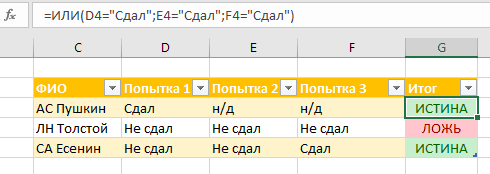
Fulfillment of the OR condition

A simple OR operator determines whether the condition given in parentheses is met and returns one of the values TRUE or FALSE. In the future, this formula can be used as a component of more difficult conditions, when, depending on what will give the value OR, this or that action will be performed.

At the same time, they can be compared as numerical indicators, using the signs >,<, =, так и поиск конкретного значения для ячейки, которое может быть текстовым. В частности, для поиска слова «Сдал» в конкретных ячейках будет использоваться формула =ИЛИ(D4= “Сдал”; E4= “Сдал”; F4= “Сдал”)

Application: One way to use this function could be to take into account the success of passing the test of three attempts, where one pass is enough for further training / participation.

Finding and Using a Value

Horizontally

Using the HLOOKUP function, we can set a search for a specific table row, and at the output get a value from another cell in the same column (one or more rows below), which corresponds to the specified condition. Moreover, the search is set either to the exact value (using the FALSE operator), or to the approximate value (with the TRUE operator), which allows the use of intervals. Syntax =HLOOKUP(lookup_value, table, row_number, interval_lookup)

Application: To calculate the bonus for a specific employee, you can set intervals, starting from which one or another percentage of profit is valid. Let's say the formula =GLOOKUP(E5;$D$1:$G$2;2;TRUE) will look in the first row of the table from the interval D1:G2 for a value approximately similar to the value from cell E5, and the result of the formula will be the output of the cell from the second row corresponding column.

Vertically

The VLOOKUP function works in a similar way - only the logic of the action is slightly different. The search will be carried out not horizontally, but vertically, that is, along the cells of one column, and the result will be taken from the specified cell of the found row.

That is, for the formula =VLOOKUP(E4;$I$3:$J$6;2;TRUE), the value of cell E4 will be compared with the cells of column I from the interval table I3:J6, and the value will be returned from the adjacent cell of column J.

Fulfillment of the IF condition

When using this function, a specific condition is specified, and then two results - one for cases where the conditions are met, and the other - vice versa. Let's say to compare funds from two columns, the following formula can be used =IF(C2>B2; “Over budget”; “Within budget”).

In addition, another function can be used as a condition, such as an OR condition and even another IF condition. At the same time, the IF functions can have from 3 to 64 possible results). As an example, =IF(D4=1, “YES”, IF(D4=2, “No”, “Maybe”)).

As a result, the value of the specified cell can also be displayed, both text and numeric. In this case, in the future it will be enough to change the value of one cell, without having to edit the formula in all places of use.

Ranking Formula

For the value of numbers, you can use the RANK formula, which will give the value of each number relative to others in a given list. In this case, the ranking can be both from a lower value towards an increase, and vice versa.

For the security of your documents, it is not superfluous to set a personal password on them.

For this function, three parameters are used - directly a number, an array or a reference to a list of numbers and order. In this case, if the order is not specified or the value is 0, then the rank is determined in descending order. Any other value for order will sort the values in ascending order.

Application: For a table with income by months, you can add a column with a ranking, and then sort by this column.

Maximum of selected values

A simple but very useful MAX formula returns the largest value from a list of values. The list itself can consist of both cells and/or their range, as well as manually entered numbers. In total, the maximum value can be searched among a list of 255 numbers.

Application: Returning to the example with ranking, instead of the rank, you can display the value of the best indicator for the selected period.

Minimum of selected values

The formula for finding the minimum values works in a similar way. Identical syntax, reverse output.

Average of selected values

There is also a formula to get the arithmetic mean from the selected list of values. However, its spelling in Russian is not so obvious. It sounds like AVERAGE, after which either specific values or cell references are indicated in brackets.

Sum of Selected Values

Finally, the most common feature that everyone who has ever used electronic Excel tables. Addition is performed using the SUM formula, and the interval or intervals of the cells whose values are to be summed are specified in brackets.

A much more interesting option is to sum the cells that meet specific criteria. To do this, use the SUMIF operator with arguments range, condition, summation range.

Application: For example, there is a list of schoolchildren who agreed to go on an excursion. Everyone has a status - whether he paid for the event or not. Thus, depending on the contents of the "Paid" column, the value from the "Cost" column will be considered or not. =SUMIF(E5:E9, "Yes", F5:F9)